Introduction to Algorithms

CS 351: Algorithms

Introduction to Algorithms

Alternative Formats

• Slides
• Outline
• PDF

Part 1: Course Introduction & Why Algorithms Matter

Welcome to Algorithms! 🚀

What We’ll Learn

• Design algorithms that solve problems
• Analyze their efficiency
• Compare different approaches
• Apply algorithmic thinking

Course Philosophy

“Perhaps the most important principle for the good algorithm designer is to refuse to be content.”

— Aho, Hopcroft, and Ullman

Our Mantra: Can we do better? 🤔

Why Study Algorithms?

1. Foundation for Computer Science 🏗️

• Routing protocols → Shortest path algorithms
• Cryptography → Number-theoretic algorithms
  
• Graphics → Geometric algorithms
• Databases → Search tree data structures
• Biology → Dynamic programming for genome similarity

2. Driver of Innovation 💡

“Performance gains due to improvements in algorithms have vastly exceeded even the dramatic performance gains due to increased processor speed.”
— Report to the White House, 2010

Interactive Demo: The Power of Algorithms

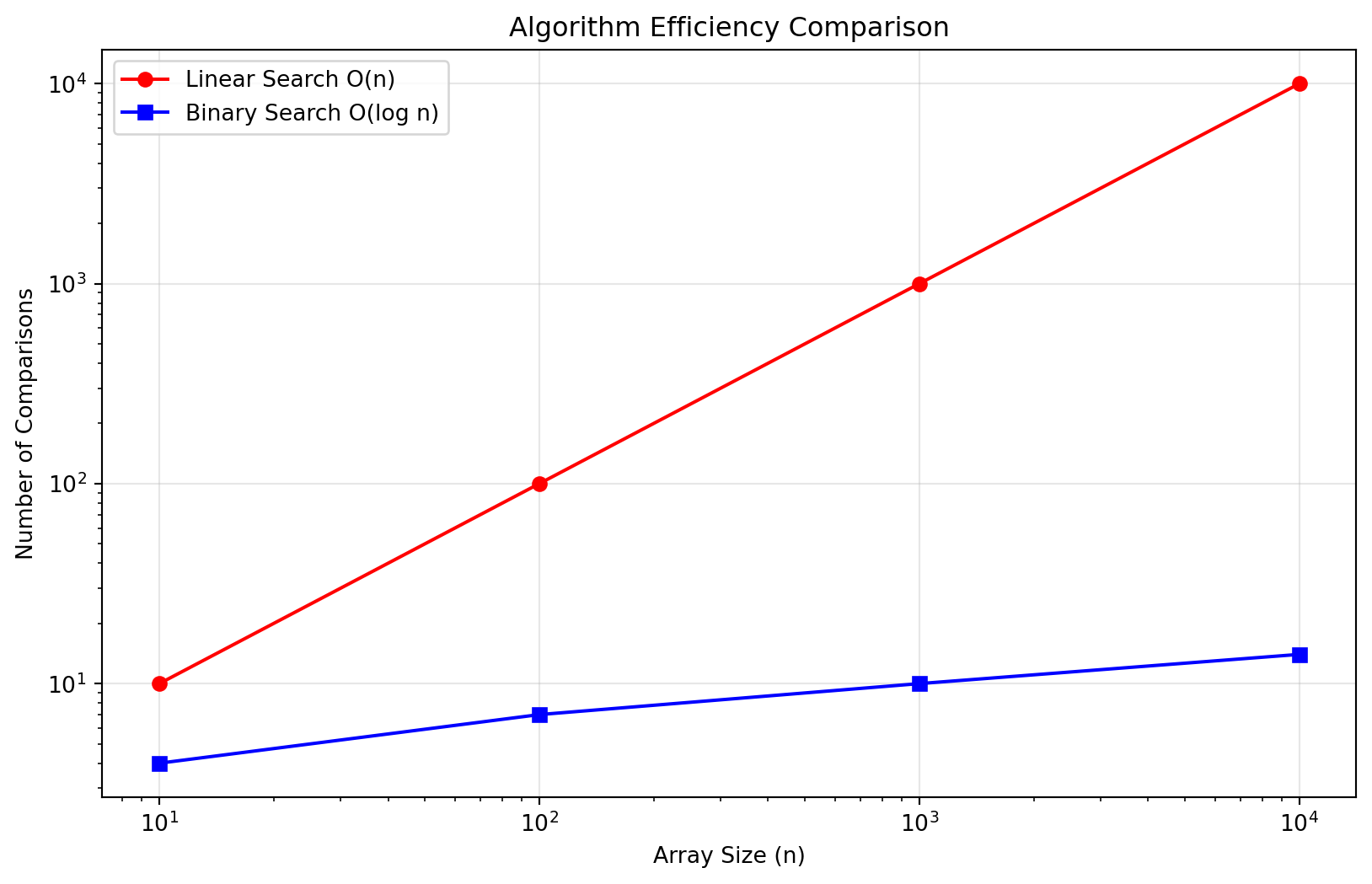
import time
import matplotlib.pyplot as plt
import numpy as np

# Simulating algorithm performance
def naive_search(arr, target):
    """O(n) linear search"""
    comparisons = 0
    for i in range(len(arr)):
        comparisons += 1
        if arr[i] == target:
            return comparisons
    return comparisons

def binary_search(arr, target):
    """O(log n) binary search"""
    comparisons = 0
    left, right = 0, len(arr) - 1
    while left <= right:
        comparisons += 1
        mid = (left + right) // 2
        if arr[mid] == target:
            return comparisons
        elif arr[mid] < target:
            left = mid + 1
        else:
            right = mid - 1
    return comparisons

# Visualization
sizes = [10, 100, 1000, 10000]
linear_comps = []
binary_comps = []

for n in sizes:
    arr = list(range(n))
    linear_comps.append(naive_search(arr, n-1))
    binary_comps.append(binary_search(arr, n-1))

plt.figure(figsize=(10, 6))
plt.plot(sizes, linear_comps, 'r-', label='Linear Search O(n)', marker='o')
plt.plot(sizes, binary_comps, 'b-', label='Binary Search O(log n)', marker='s')
plt.xlabel('Array Size (n)')
plt.ylabel('Number of Comparisons')
plt.title('Algorithm Efficiency Comparison')
plt.legend()
plt.xscale('log')
plt.yscale('log')
plt.grid(True, alpha=0.3)
plt.show()

🎯 Quick Quiz 1

Question: You have 1 million sorted numbers. How many comparisons does binary search need in the worst case?

Answer: About 20 comparisons!

- $\log_2(1,000,000) \approx 20$
- Linear search would need 1,000,000 comparisons!

Integer Multiplication: A First Example

The Problem

• Input: Two n-digit numbers, x and y
• Output: Their product x · y

Grade-School Algorithm

    5678
  × 1234
  ------
   22712  (5678 × 4)
  17034   (5678 × 3, shifted)
  11356   (5678 × 2, shifted)
  5678    (5678 × 1, shifted)
  ------
 7006652

Time Complexity: ~\(n^2\) operations
Can we do better? 🤔

Karatsuba’s Breakthrough (1960)

The Clever Trick 🎩

Split numbers in half: \(x = 10^{n/2} \cdot a + b\)

Naive approach: 4 multiplications - \(a \cdot c\) - \(a \cdot d\)
- \(b \cdot c\) - \(b \cdot d\)

Karatsuba: Only 3 multiplications! 1. \(P_1 = a \cdot c\) 2. \(P_2 = b \cdot d\) 3. \(P_3 = (a+b) \cdot (c+d)\)

Then: \(ad + bc = P_3 - P_1 - P_2\)

Live Coding: Karatsuba Implementation

def karatsuba(x, y):
    """Karatsuba multiplication algorithm"""
    # Base case
    if x < 10 or y < 10:
        return x * y
    
    # Calculate size of numbers
    n = max(len(str(x)), len(str(y)))
    half = n // 2
    
    # Split the numbers
    a = x // (10 ** half)
    b = x % (10 ** half)
    c = y // (10 ** half)
    d = y % (10 ** half)
    
    # Three recursive calls
    ac = karatsuba(a, c)
    bd = karatsuba(b, d)
    ad_plus_bc = karatsuba(a + b, c + d) - ac - bd
    
    # Combine results
    return ac * (10 ** (2 * half)) + ad_plus_bc * (10 ** half) + bd

# Test it!
x = 1234
y = 5678
result = karatsuba(x, y)
print(f"{x} × {y} = {result}")
print(f"Verification: {x * y == result}")

1234 × 5678 = 7006652
Verification: True

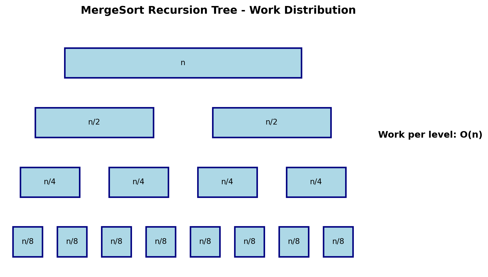
Part 2: Algorithm Fundamentals with MergeSort

The Sorting Problem

Definition

• Input: Array of n numbers in arbitrary order
• Output: Same numbers, sorted from smallest to largest

Example

Input:  [5, 4, 1, 8, 7, 2, 6, 3]
Output: [1, 2, 3, 4, 5, 6, 7, 8]

Simple Approaches

• SelectionSort: Find minimum, repeat → O(n²)
• InsertionSort: Build sorted portion → O(n²)
  
• BubbleSort: Swap adjacent pairs → O(n²)

Can we do better? 🚀

Divide and Conquer Paradigm

The Strategy

1. Divide the problem into smaller subproblems
2. Conquer the subproblems recursively
3. Combine the solutions

MergeSort Overview

graph TD
    A[5,4,1,8,7,2,6,3] --> B[5,4,1,8]
    A --> C[7,2,6,3]
    B --> D[5,4]
    B --> E[1,8]
    C --> F[7,2]
    C --> G[6,3]
    D --> H[1,4,5,8]
    E --> H
    F --> I[2,3,6,7]
    G --> I
    H --> J[1,2,3,4,5,6,7,8]
    I --> J

Interactive MergeSort Visualization

def merge(left, right):
    """Merge two sorted arrays"""
    result = []
    i = j = 0
    
    # Merge process with step tracking
    steps = []
    while i < len(left) and j < len(right):
        if left[i] <= right[j]:
            result.append(left[i])
            steps.append(f"Compare {left[i]} ≤ {right[j]}: Take {left[i]} from left")
            i += 1
        else:
            result.append(right[j])
            steps.append(f"Compare {left[i]} > {right[j]}: Take {right[j]} from right")
            j += 1
    
    # Add remaining elements
    result.extend(left[i:])
    result.extend(right[j:])
    
    return result, steps

def mergesort_visual(arr, depth=0):
    """MergeSort with visualization"""
    indent = "  " * depth
    print(f"{indent}Sorting: {arr}")
    
    if len(arr) <= 1:
        return arr
    
    mid = len(arr) // 2
    left = mergesort_visual(arr[:mid], depth + 1)
    right = mergesort_visual(arr[mid:], depth + 1)
    
    result, steps = merge(left, right)
    print(f"{indent}Merging {left} + {right} = {result}")
    
    return result

# Demo
test_array = [5, 4, 1, 8, 7, 2, 6, 3]
print("MergeSort Trace:")
sorted_array = mergesort_visual(test_array)
print(f"\nFinal result: {sorted_array}")

MergeSort Trace:
Sorting: [5, 4, 1, 8, 7, 2, 6, 3]
  Sorting: [5, 4, 1, 8]
    Sorting: [5, 4]
      Sorting: [5]
      Sorting: [4]
    Merging [5] + [4] = [4, 5]
    Sorting: [1, 8]
      Sorting: [1]
      Sorting: [8]
    Merging [1] + [8] = [1, 8]
  Merging [4, 5] + [1, 8] = [1, 4, 5, 8]
  Sorting: [7, 2, 6, 3]
    Sorting: [7, 2]
      Sorting: [7]
      Sorting: [2]
    Merging [7] + [2] = [2, 7]
    Sorting: [6, 3]
      Sorting: [6]
      Sorting: [3]
    Merging [6] + [3] = [3, 6]
  Merging [2, 7] + [3, 6] = [2, 3, 6, 7]
Merging [1, 4, 5, 8] + [2, 3, 6, 7] = [1, 2, 3, 4, 5, 6, 7, 8]

Final result: [1, 2, 3, 4, 5, 6, 7, 8]

Analyzing MergeSort: Recursion Tree

Key Insights 🔍

At each level j: - \(2^j\) subproblems - Each of size \(n/2^j\) - Work per level: \(O(n)\)

Total analysis: - Tree depth: \(\log_2 n\) - Levels: \(\log_2 n + 1\) - Total work: \(O(n \log n)\)

# Visualizing recursion tree work
import matplotlib.pyplot as plt

levels = 4
fig, ax = plt.subplots(figsize=(10, 6))

for level in range(levels):
    num_nodes = 2**level
    node_size = 100 / num_nodes
    work = f"n/{2**level}" if level > 0 else "n"
    
    for node in range(num_nodes):
        x = (node + 0.5) * (100 / num_nodes)
        y = (levels - level - 1) * 20
        
        # Draw node
        rect = plt.Rectangle((x - node_size/3, y), node_size/1.5, 10, 
                            fill=True, facecolor='lightblue', 
                            edgecolor='navy', linewidth=2)
        ax.add_patch(rect)
        ax.text(x, y + 5, work, ha='center', va='center', fontsize=10)

ax.text(105, levels * 10, f"Work per level: O(n)", fontsize=12, weight='bold')
ax.set_xlim(0, 120)
ax.set_ylim(-5, levels * 20)
ax.axis('off')
ax.set_title('MergeSort Recursion Tree - Work Distribution', fontsize=14, weight='bold')
plt.show()

🎯 Quick Quiz 2

Question: If MergeSort takes 1 second to sort 1 million items, approximately how long for 2 million items?

Answer: About 2.02 seconds! - Time complexity: \(O(n \log n)\) - \(2n \log(2n) = 2n(\log n + 1) \approx 2n \log n + 2n\) - Roughly doubles (plus a tiny bit more)

Hands-On Exercise: Trace MergeSort

Your Turn! Trace MergeSort on: [3, 7, 1, 4]

1. Draw the recursion tree
2. Show the merge steps
3. Count total comparisons

Solution:

       [3,7,1,4]
       /        \
    [3,7]      [1,4]
    /   \      /   \
  [3]   [7]  [1]   [4]
    \   /      \   /
    [3,7]      [1,4]
       \        /
       [1,3,4,7]

Total comparisons: ~5

Part 3: Big-O Notation & Asymptotic Analysis

Why Asymptotic Notation?

The Challenge

How do we compare algorithms across: - Different programming languages? - Different hardware? - Different compilers? - Different input sizes?

The Solution: Big-O Notation

Focus on growth rate, not exact counts!

Suppress: - Constant factors (system-dependent) - Lower-order terms (irrelevant for large n)

Big-O Intuition

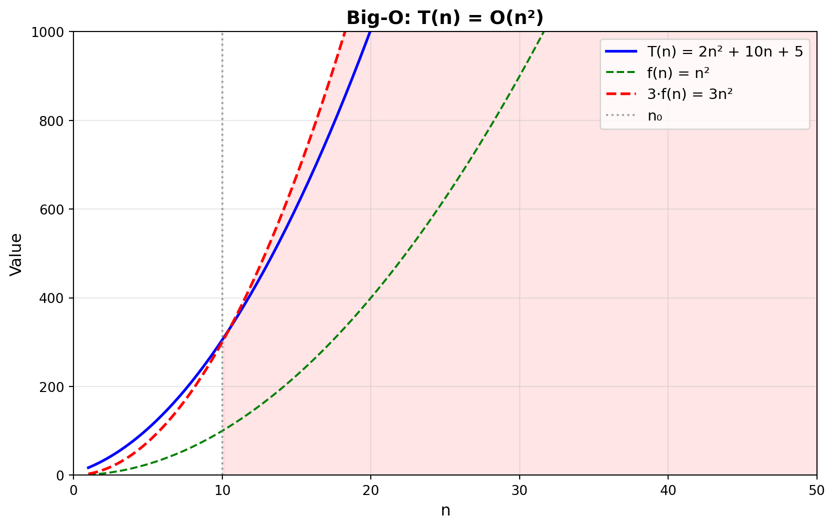
Formal Definition of Big-O

Mathematical Definition

\(T(n) = O(f(n))\) if and only if there exist positive constants \(c\) and \(n_0\) such that:

\[T(n) \leq c \cdot f(n) \text{ for all } n \geq n_0\]

In Plain English

“\(T(n)\) is eventually bounded above by a constant multiple of \(f(n)\)”

Visual Interpretation

Interactive Big-O Practice

def analyze_code_complexity(code_type):
    """Analyze different code patterns"""
    
    examples = {
        'constant': {
            'code': 'x = arr[0] + arr[n-1]',
            'complexity': 'O(1)',
            'explanation': 'Fixed number of operations'
        },
        'linear': {
            'code': 'for i in range(n):\n    process(arr[i])',
            'complexity': 'O(n)',
            'explanation': 'Single loop through n elements'
        },
        'quadratic': {
            'code': 'for i in range(n):\n    for j in range(n):\n        process(arr[i], arr[j])',
            'complexity': 'O(n²)',
            'explanation': 'Nested loops, n × n iterations'
        },
        'logarithmic': {
            'code': 'while n > 1:\n    n = n // 2\n    process()',
            'complexity': 'O(log n)',
            'explanation': 'Halving n each iteration'
        }
    }
    
    example = examples.get(code_type, examples['linear'])
    print(f"Code Pattern:\n{example['code']}\n")
    print(f"Complexity: {example['complexity']}")
    print(f"Reason: {example['explanation']}")
    return example

# Try different patterns
print("=" * 50)
print("ANALYZING CODE COMPLEXITY")
print("=" * 50)
for pattern in ['constant', 'logarithmic', 'linear', 'quadratic']:
    analyze_code_complexity(pattern)
    print("-" * 50)

==================================================
ANALYZING CODE COMPLEXITY
==================================================
Code Pattern:
x = arr[0] + arr[n-1]

Complexity: O(1)
Reason: Fixed number of operations
--------------------------------------------------
Code Pattern:
while n > 1:
    n = n // 2
    process()

Complexity: O(log n)
Reason: Halving n each iteration
--------------------------------------------------
Code Pattern:
for i in range(n):
    process(arr[i])

Complexity: O(n)
Reason: Single loop through n elements
--------------------------------------------------
Code Pattern:
for i in range(n):
    for j in range(n):
        process(arr[i], arr[j])

Complexity: O(n²)
Reason: Nested loops, n × n iterations
--------------------------------------------------

Big-O Family: Ω and Θ

Big-O

Upper bound (≤) \[T(n) = O(f(n))\] “At most this fast”

Big-Omega (Ω)

Lower bound (≥) \[T(n) = \Omega(f(n))\] “At least this slow”

Big-Theta (Θ)

Tight bound (=) \[T(n) = \Theta(f(n))\] “Exactly this rate”

Example: MergeSort - \(T(n) = O(n \log n)\) ✓ (upper bound) - \(T(n) = \Omega(n \log n)\) ✓ (lower bound)
- \(T(n) = \Theta(n \log n)\) ✓ (tight bound)

🎯 Quick Quiz 3: Big-O Challenge

Match the code to its complexity:

# Code A
for i in range(n):
    for j in range(i+1, n):
        process(i, j)

# Code B  
i = n
while i > 0:
    process(i)
    i = i // 3

# Code C
for i in range(n):
    binary_search(arr, target)

Options: O(n²), O(n log n), O(log n)

Answers: - Code A: O(n²) - nested loops with ~n²/2 iterations - Code B: O(log n) - dividing by 3 each time - Code C: O(n log n) - n iterations × log n per search

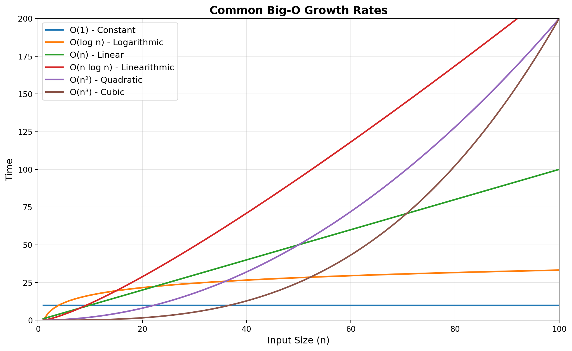
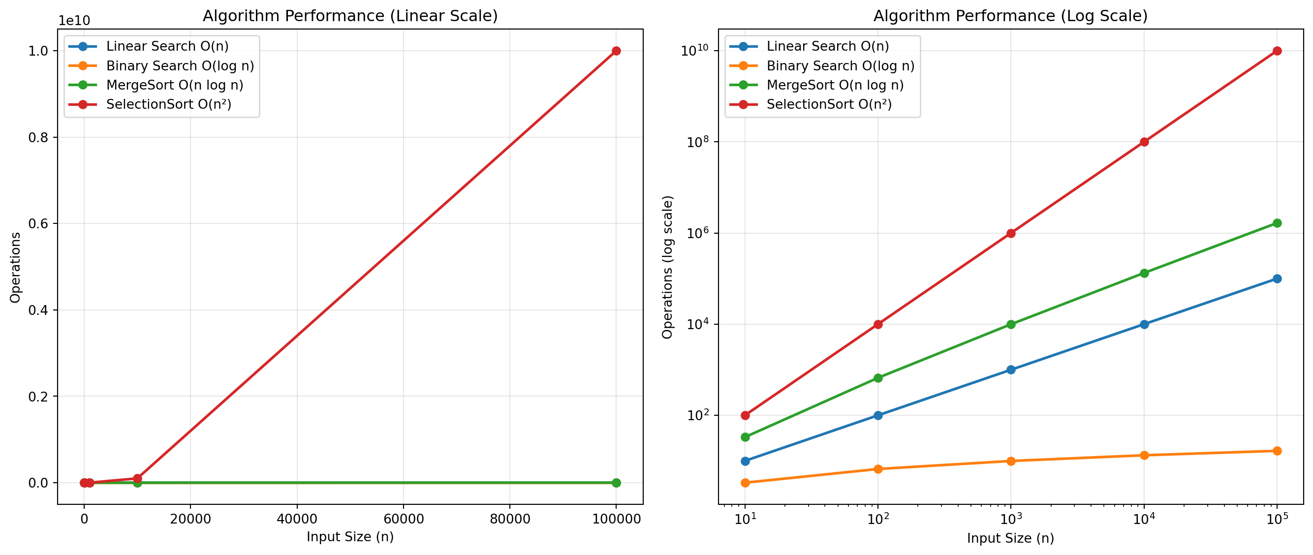
Common Complexity Classes

Complexity	Name	Example Algorithm	1000 items
O(1)	Constant	Array access	1 op
O(log n)	Logarithmic	Binary search	~10 ops
O(n)	Linear	Linear search	1,000 ops
O(n log n)	Linearithmic	MergeSort	~10,000 ops
O(n²)	Quadratic	Selection sort	1,000,000 ops
O(2ⁿ)	Exponential	Subset generation	2¹⁰⁰⁰ ops 😱

Key Insight: For large n, even small improvements in complexity class yield massive speedups!

Practice Problem: Analyzing Nested Loops

Analyze this code:

def mystery(n):
    count = 0
    for i in range(n):
        j = 1
        while j < n:
            count += 1
            j = j * 2
    return count

What’s the complexity?

Solution: - Outer loop: n iterations - Inner loop: log₂(n) iterations (doubling j) - Total: O(n log n)

Real-World Performance Impact

Lab Exercise: Implement & Analyze

Your Mission

1. Implement these sorting algorithms:

   • SelectionSort (O(n²))
   • MergeSort (O(n log n))

2. Measure actual running times for n = [100, 500, 1000, 5000]

3. Plot results and verify theoretical predictions

import time

def time_algorithm(algo, arr):
    start = time.time()
    algo(arr.copy())
    return time.time() - start

# Starter code
def selection_sort(arr):
    # TODO: Implement
    pass

def merge_sort(arr):
    # TODO: Implement  
    pass

Key Takeaways 🎓

1. Algorithms matter - Can be difference between seconds and years!

2. Divide & Conquer - Break problems into smaller subproblems

3. Asymptotic analysis - Focus on growth rate, not exact counts

4. Big-O notation - Universal language for algorithm efficiency

5. MergeSort beats O(n²) - O(n log n) is dramatically faster for large n

Next Week Preview

• QuickSort and randomized algorithms
• The Master Method for analyzing recursions
• Lower bounds and optimality

Discussion & Questions

Let’s Discuss! 💬

Conceptual Questions

- Why does log n grow so slowly?
- When do constants matter?
- Is O(n) always better than O(n²)?

Practical Questions - Real-world algorithm choice? - Space vs. time tradeoffs? - Best practices for analysis?

Resources

• Visualizing Algorithms
• Big-O Cheat Sheet
• Practice problems on LeetCode

Homework & Practice

This Week’s Assignments

1. Reading: Roughgarden Ch. 1-2 (complete)
2. Implementation:
   • Karatsuba multiplication
   • MergeSort with step counter
3. Analysis Problems:
   • Prove T(n) = 3n² + 2n = O(n²)
   • Find tight bounds for 5 given functions
4. Challenge: Implement 3-way MergeSort

---

Next next class: QuickSort! 🚀

Remember: Can we do better?