Pathfinding Algorithms

CS 351: Analysis of Algorithms

Author

Affiliation

Lucas P. Cordova, Ph.D.

Willamette University

Abstract

This lecture reviews the three pathfinding algorithms we’ll use in Project 2: Greedy Best-First Search, Dijkstra’s Algorithm, and A*.

Introduction

What Are Pathfinding Algorithms?

Pathfinding algorithms find the optimal or near-optimal route between two points in a graph.

Applications:

GPS navigation and route planning
Video game AI and character movement
Network routing protocols
Robotics path planning
Logistics and delivery optimization

Why Multiple Algorithms?

Different algorithms make different trade-offs:

Speed vs. Optimality - Fast approximation vs. guaranteed shortest path
Memory usage - How much information needs to be stored
Use of heuristics - Leveraging domain knowledge for efficiency

Today we’ll review the three fundamental approaches to pathfinding on the same problem.

The Problem Setup

Our Example Graph

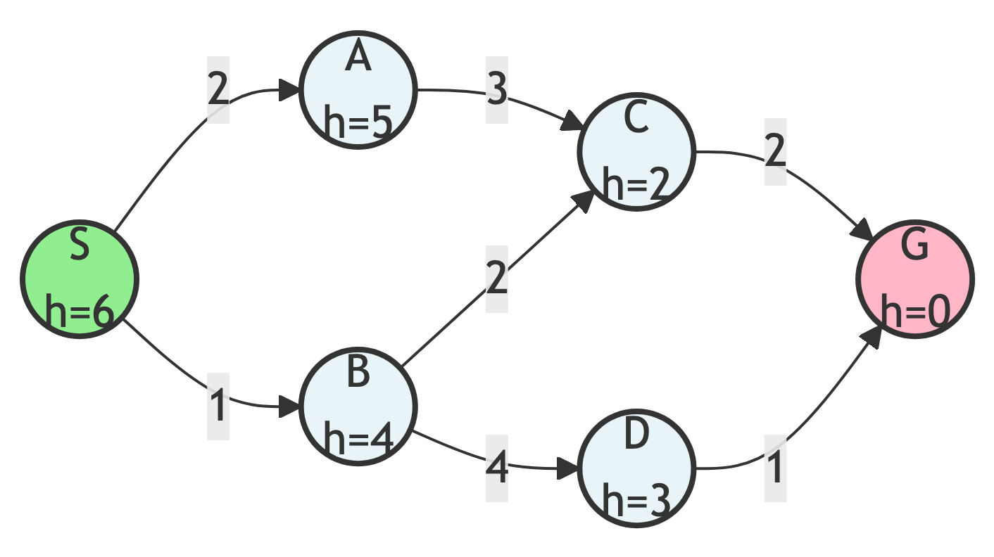
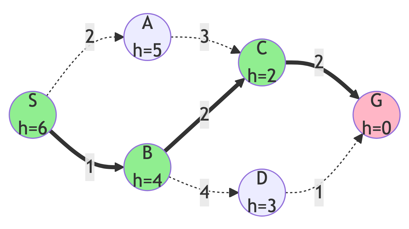
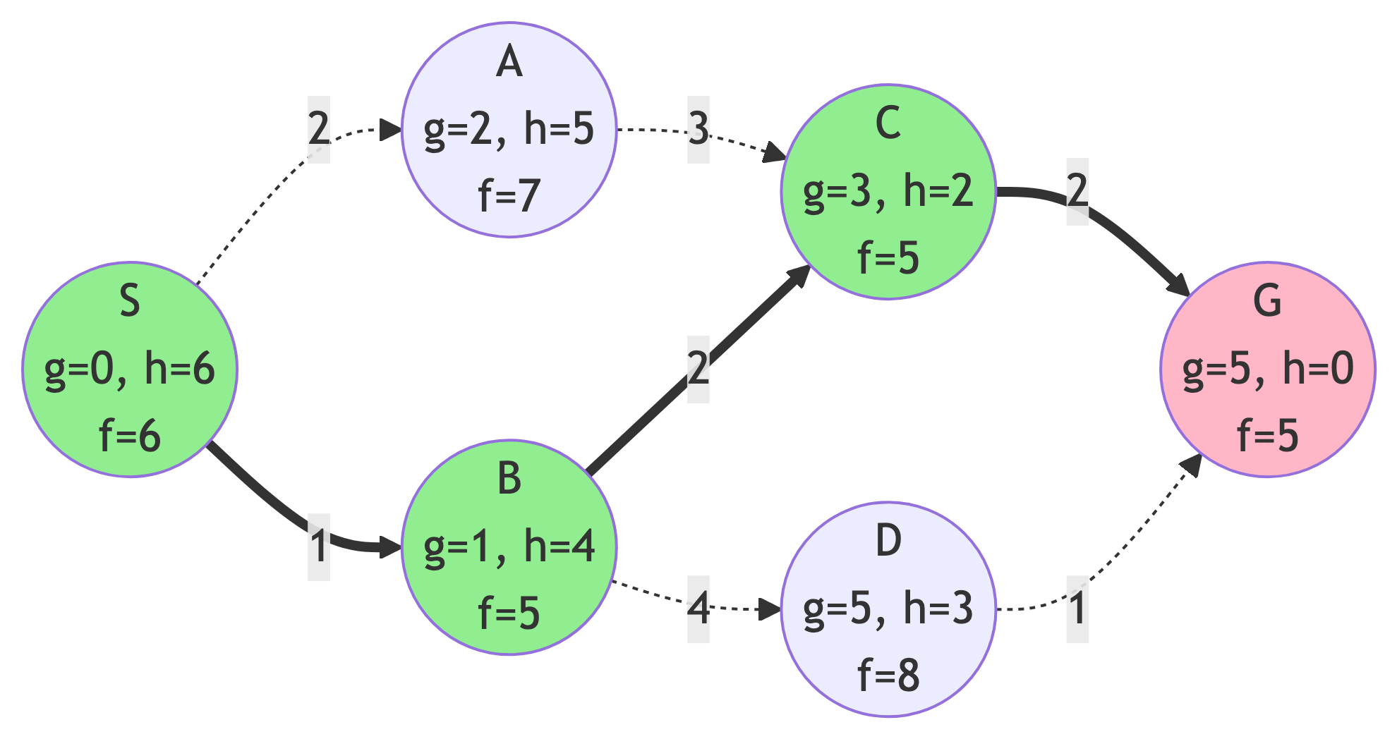
We’ll use a simple graph with 6 nodes to illustrate each algorithm:

Goal: Find a path from S (start) to G (goal)

Graph Components

Nodes:

S (Start) - our starting point
A, B, C, D - intermediate nodes
G (Goal) - our destination

Edge Costs:

The numbers on edges represent the actual cost to traverse the edge

Heuristic Values h(n):

Estimated distance from each node to goal (shown below node names)
This is a heuristic, an estimate of the remaining distance to the goal

Graph Data Table

Edge	Cost	Node	h(n)
S → A	2	S	6
S → B	1	A	5
A → C	3	B	4
B → C	2	C	2
B → D	4	D	3
C → G	2	G	0
D → G	1

Note: The heuristic h(n) represents an estimate of the remaining distance to the goal.

Greedy Best-First Search

Algorithm Overview

Strategy:

Always expand the node that appears closest to the goal based on the heuristic function h(n).

Key Characteristics:

Uses only the heuristic h(n), ignoring actual path cost
Greedy approach - makes locally optimal choices
Fast but not guaranteed to find the optimal path
Can be misled by poor heuristics

Greedy BFS: The Idea

Think of it like:

Following the “scent” directly toward the goal, always choosing the path that seems to lead most directly there.

Analogy:

Like a person lost in a forest who always walks in the direction that feels closest to home, without considering how difficult the terrain might be.

Greedy BFS Pseudocode

function GreedyBestFirstSearch(start, goal):
    frontier = PriorityQueue()
    frontier.add(start, h(start))
    explored = empty set
    
    while frontier is not empty:
        current = frontier.pop()  # Lowest h(n)
        
        if current == goal:
            return path
        
        explored.add(current)
        
        for each neighbor of current:
            if neighbor not in explored:
                frontier.add(neighbor, h(neighbor))
    
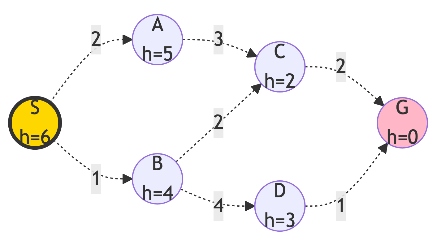
    return failure

Step 0: Initialize

Starting State:

Frontier: {S (h=6)}
Explored: {}
Current path: None

Current node: S (highlighted in gold)

Step 1: Expand S

Action:

Explore neighbors of S

Updates:

Frontier: {B (h=4), A (h=5)}
Explored: {S}
B has lower h-value, so it will be expanded next

Step 2: Expand B

Action:

B has the lowest heuristic (h=4)

Updates:

Frontier: {C (h=2), D (h=3), A (h=5)}
Explored: {S, B}
C has the lowest h-value

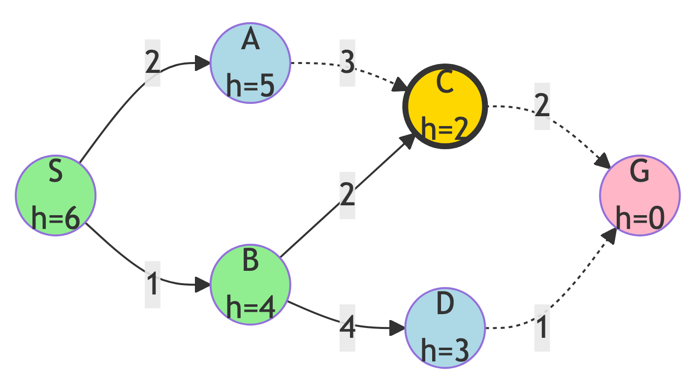
Step 3: Expand C

Action:

C has the lowest heuristic (h=2)

Updates:

Frontier: {G (h=0), D (h=3), A (h=5)}
Explored: {S, B, C}
G is now in frontier!

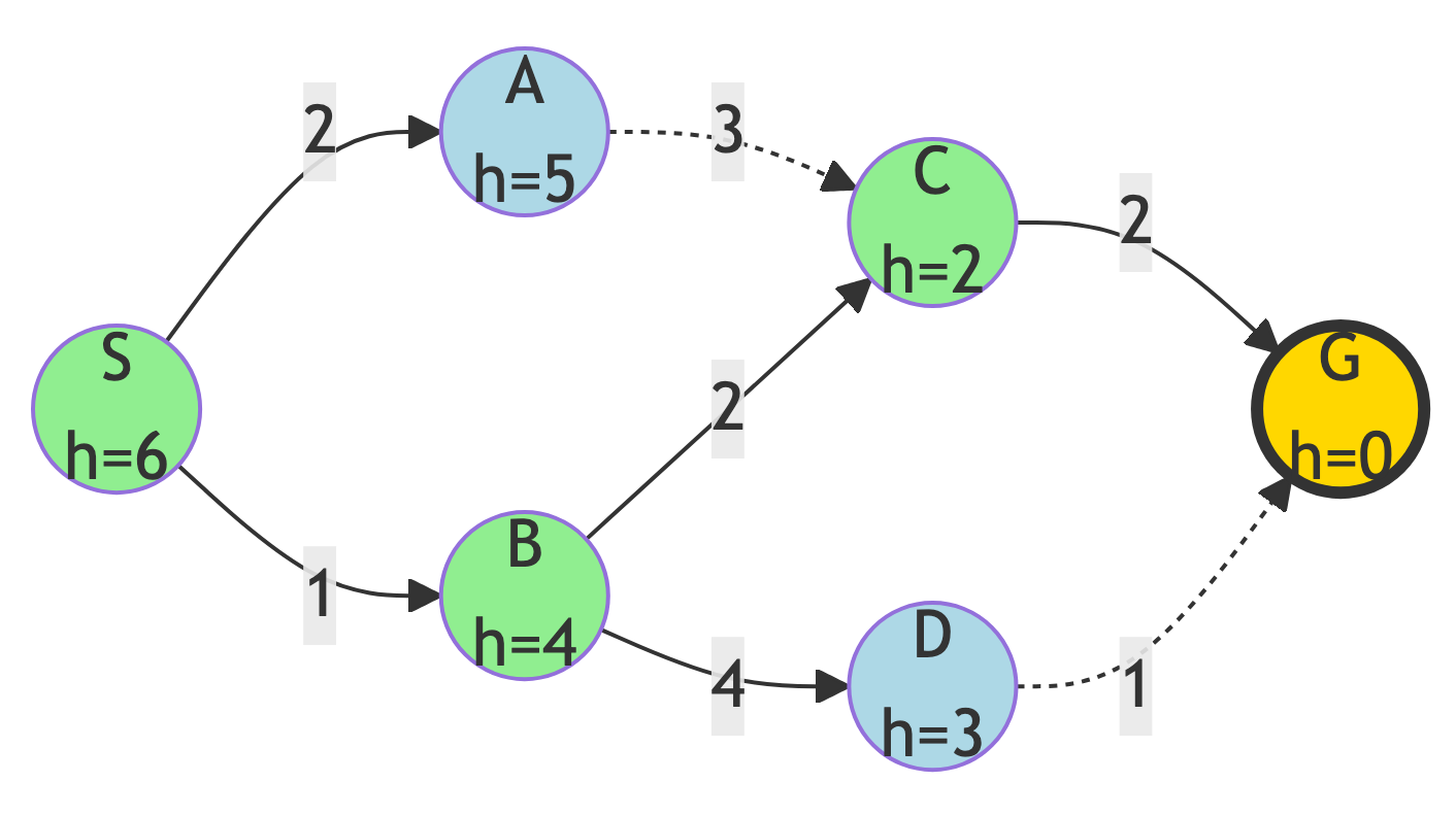
Step 4: Reach Goal

Result:

G has h=0 (lowest possible), expand it and find the goal!

Path Found:

S → B → C → G

Path Cost:

1 + 2 + 2 = 5

Greedy BFS Results

Summary:

Path: S → B → C → G
Cost: 5
Nodes Explored: 4 (S, B, C, G)
Optimal? We’ll see…

Observation:

The algorithm followed the heuristic values greedily, always choosing the node that seemed closest to the goal.

Dijkstra’s Algorithm

Algorithm Overview

Strategy:

Expand nodes in order of their actual distance g(n) from the start, guaranteeing the shortest path.

Key Characteristics:

Uses actual path cost g(n), ignoring heuristics
Guarantees optimal solution
More thorough exploration than Greedy BFS
Uniform cost search variant

Dijkstra’s Algorithm: The Idea

Think of it like:

Exploring all paths systematically by distance, like ripples expanding in water.

Analogy:

Like carefully measuring every possible route with a measuring tape, always extending the shortest path found so far.

Dijkstra Pseudocode

function Dijkstra(start, goal):
    frontier = PriorityQueue()
    frontier.add(start, 0)
    g_scores = {start: 0}
    explored = empty set
    
    while frontier is not empty:
        current = frontier.pop()  # Lowest g(n)
        
        if current == goal:
            return path
        
        explored.add(current)
        
        for each neighbor of current with cost:
            tentative_g = g[current] + cost
            if neighbor not in explored or 
               tentative_g < g[neighbor]:
                g[neighbor] = tentative_g
                frontier.add(neighbor, tentative_g)
    
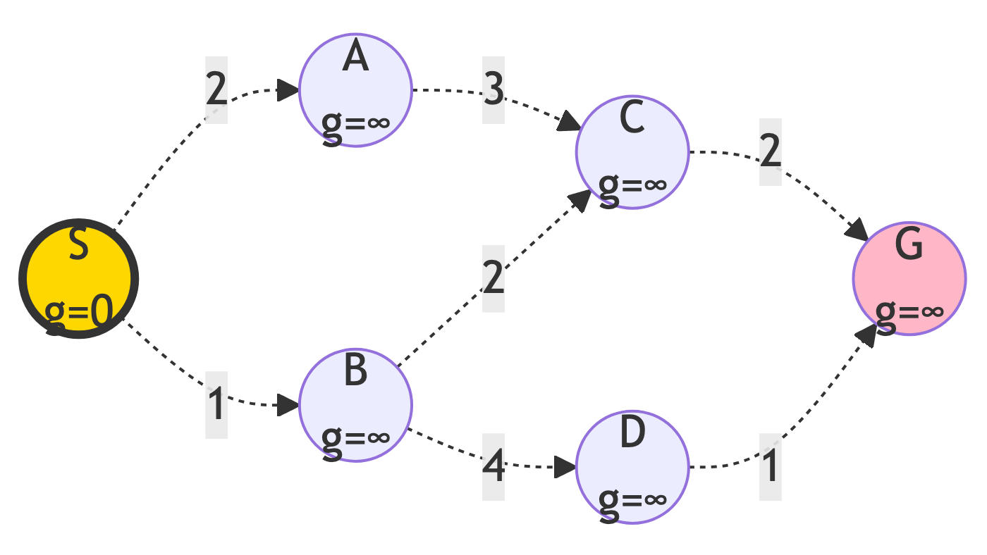
    return failure

Step 0: Initialize

Starting State:

Frontier: {S (g=0)}
g-scores: {S: 0}
Explored: {}

All nodes start with g=∞ except start

Step 1: Expand S

Action:

Explore S and update neighbors

g-score Updates:

g(A) = 0 + 2 = 2
g(B) = 0 + 1 = 1

New State:

Frontier: {B (g=1), A (g=2)}
Explored: {S}

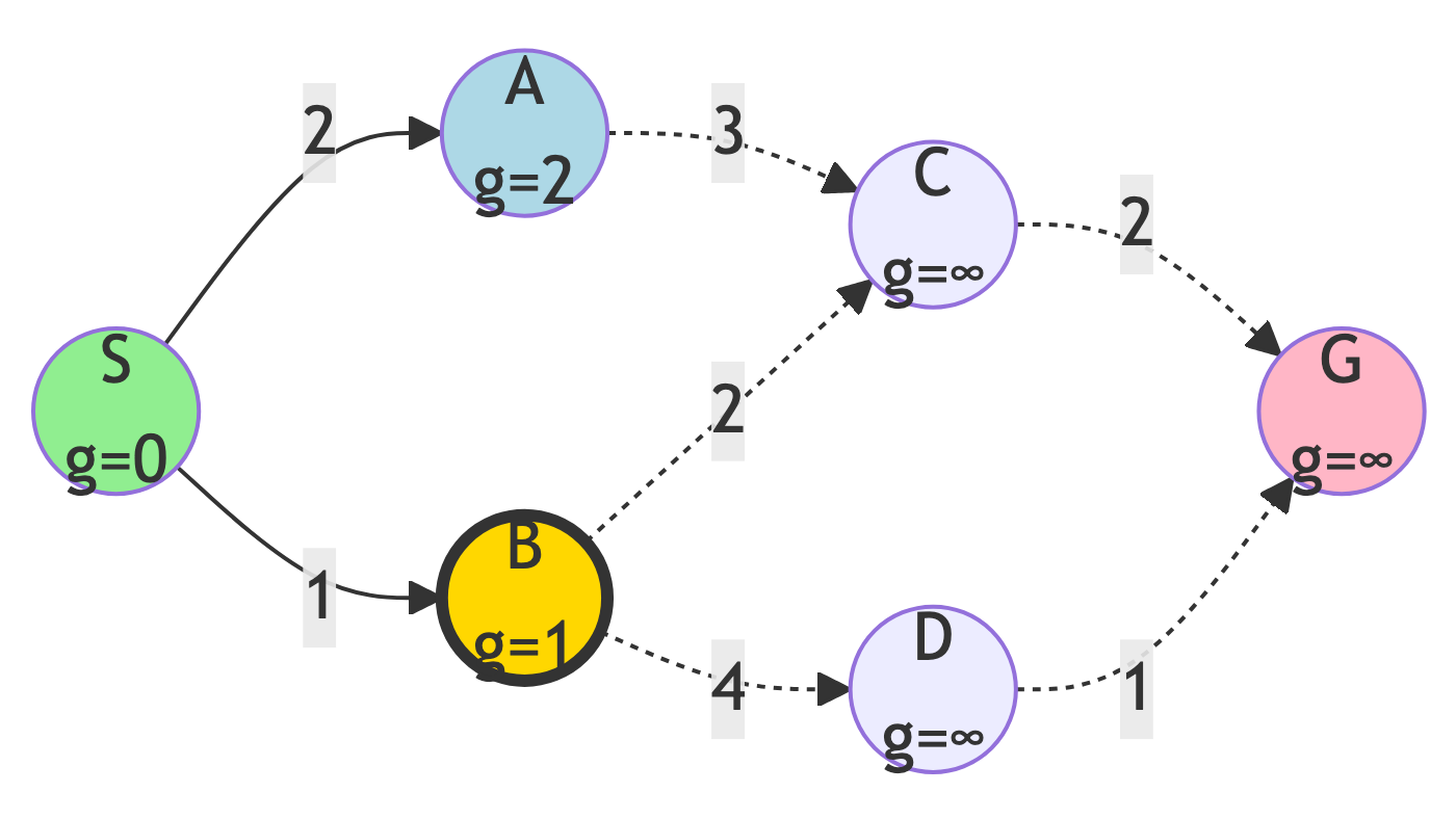
Step 2: Expand B

Action:

B has lowest g-score (g=1)

g-score Updates:

g(C) = 1 + 2 = 3
g(D) = 1 + 4 = 5

New State:

Frontier: {A (g=2), C (g=3), D (g=5)}
Explored: {S, B}

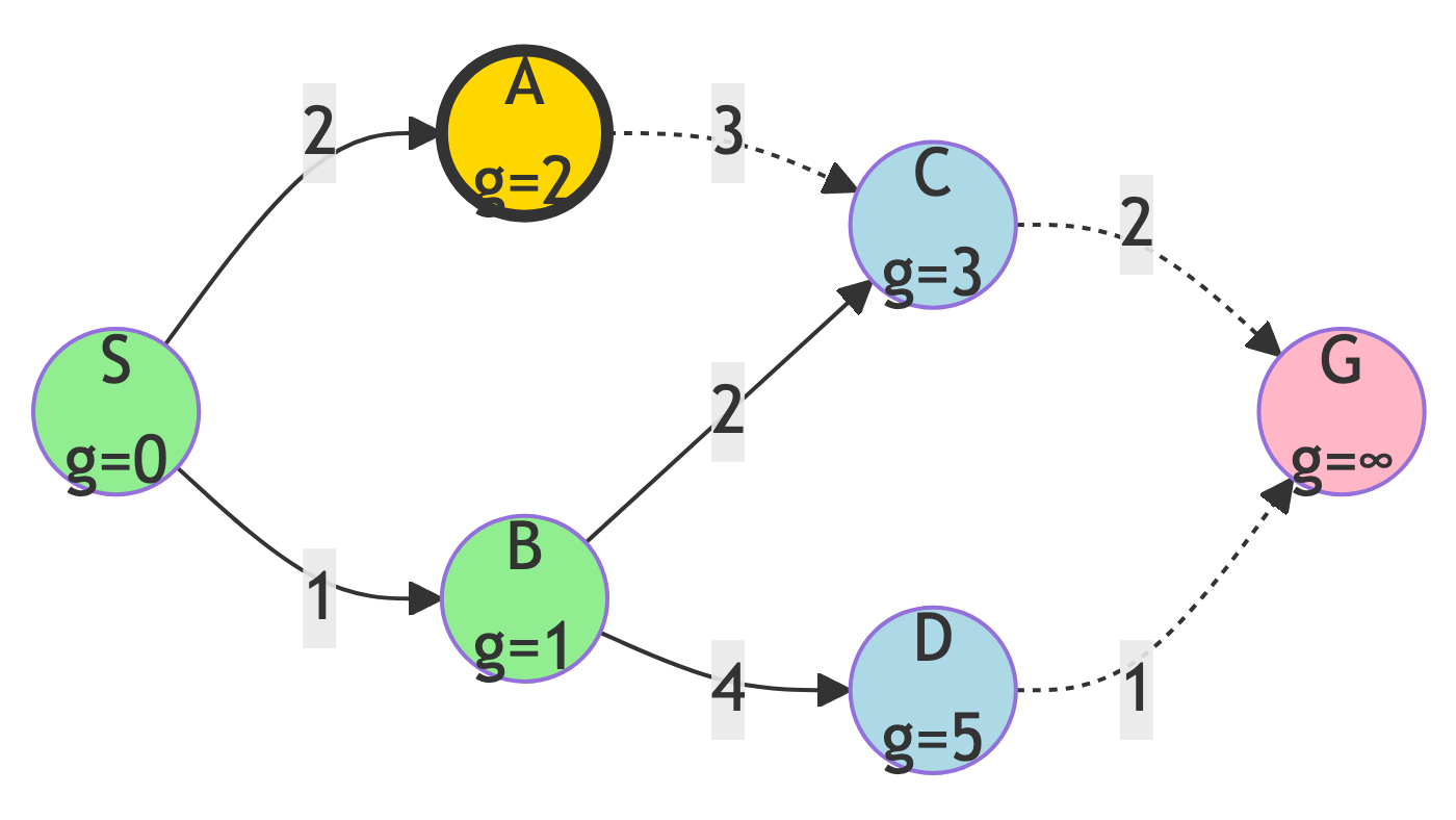
Step 3: Expand A

Action:

A has lowest g-score (g=2)

g-score Updates:

g(C) = 2 + 3 = 5 (no update, 3 is better)

New State:

Frontier: {C (g=3), D (g=5)}
Explored: {S, B, A}

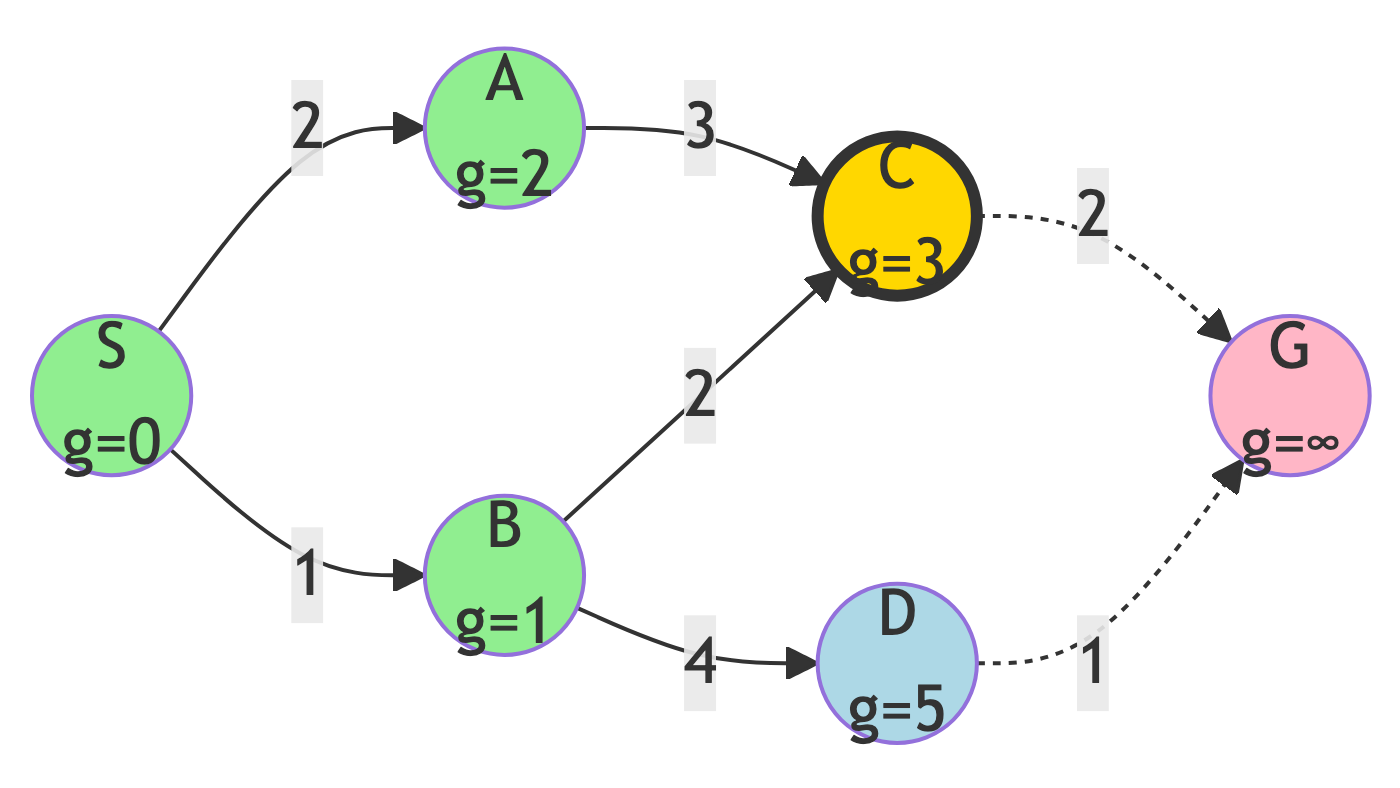
Step 4: Expand C

Action:

C has lowest g-score (g=3)

g-score Updates:

g(G) = 3 + 2 = 5

New State:

Frontier: {D (g=5), G (g=5)}
Explored: {S, B, A, C}
Tie between D and G!

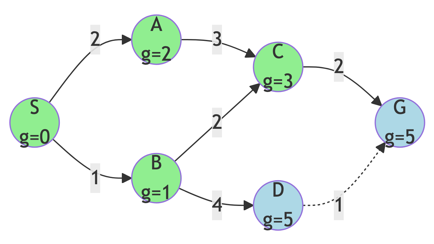
Step 5: Expand D (or G)

Action:

Break tie arbitrarily - let’s expand D first

g-score Updates:

g(G) = 5 + 1 = 6 (no update, 5 is better!)

New State:

Frontier: {G (g=5)}
Explored: {S, B, A, C, D}

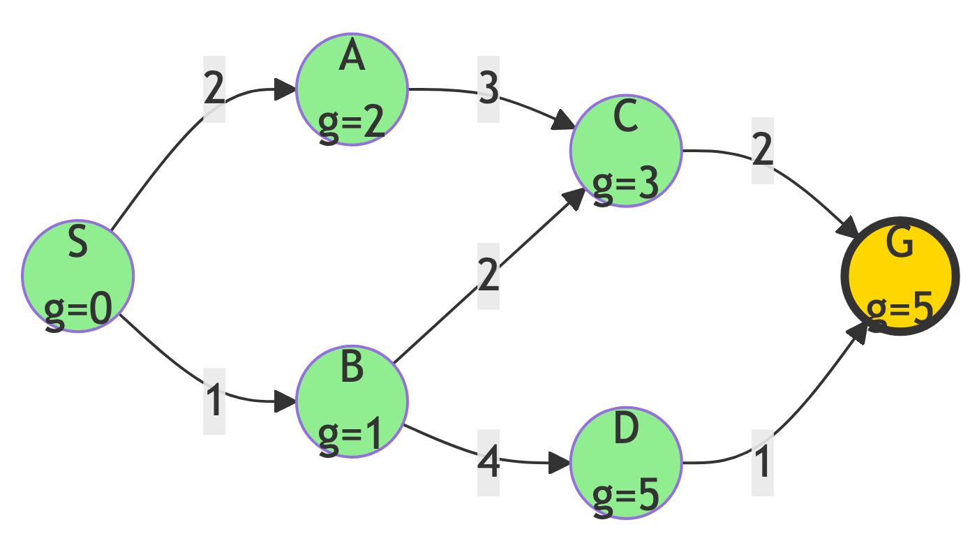
Step 6: Reach Goal

Result:

G is expanded - goal reached!

Path Found:

S → B → C → G

Path Cost:

1 + 2 + 2 = 5

Dijkstra Results

Summary:

Path: S → B → C → G
Cost: 5
Nodes Explored: 6 (S, B, A, C, D, G)
Optimal? YES - guaranteed!

Observation:

Dijkstra explored more nodes than Greedy BFS but found the same path. The key difference: Dijkstra guarantees this is optimal.

Why Is This Path Optimal?

Alternative Path Analysis:

S → A → C → G = 2 + 3 + 2 = 7 (worse)
S → B → D → G = 1 + 4 + 1 = 6 (worse)
S → B → C → G = 1 + 2 + 2 = 5 (best!)

Dijkstra checked all possibilities systematically and confirmed 5 is the minimum cost.

A* Search Algorithm

Algorithm Overview

Strategy:

Combine actual cost g(n) and heuristic h(n) using evaluation function f(n) = g(n) + h(n)

Key Characteristics:

Uses both actual cost and heuristic information
Optimal when heuristic is admissible (never overestimates)
More efficient than Dijkstra with good heuristics
Best of both worlds

A* Search: The Idea

Think of it like:

A smart explorer who considers both how far they’ve traveled AND how far they estimate they still need to go.

Analogy:

Like planning a road trip where you consider both the miles already driven and your GPS estimate of remaining distance.

A* Pseudocode

function AStar(start, goal):
    frontier = PriorityQueue()
    frontier.add(start, h(start))
    g_scores = {start: 0}
    explored = empty set
    
    while frontier is not empty:
        current = frontier.pop()  # Lowest f(n)
        
        if current == goal:
            return path
        
        explored.add(current)
        
        for each neighbor of current with cost:
            tentative_g = g[current] + cost
            if neighbor not in explored or 
               tentative_g < g[neighbor]:
                g[neighbor] = tentative_g
                f[neighbor] = g[neighbor] + h[neighbor]
                frontier.add(neighbor, f[neighbor])
    
    return failure

The f(n) Function

Evaluation Function:

f(n) = g(n) + h(n)

Components:

g(n) = actual cost from start to node n
h(n) = estimated cost from node n to goal
f(n) = estimated total cost of path through n

Intuition:

We want to explore paths that have both low actual cost so far AND promise to reach the goal efficiently.

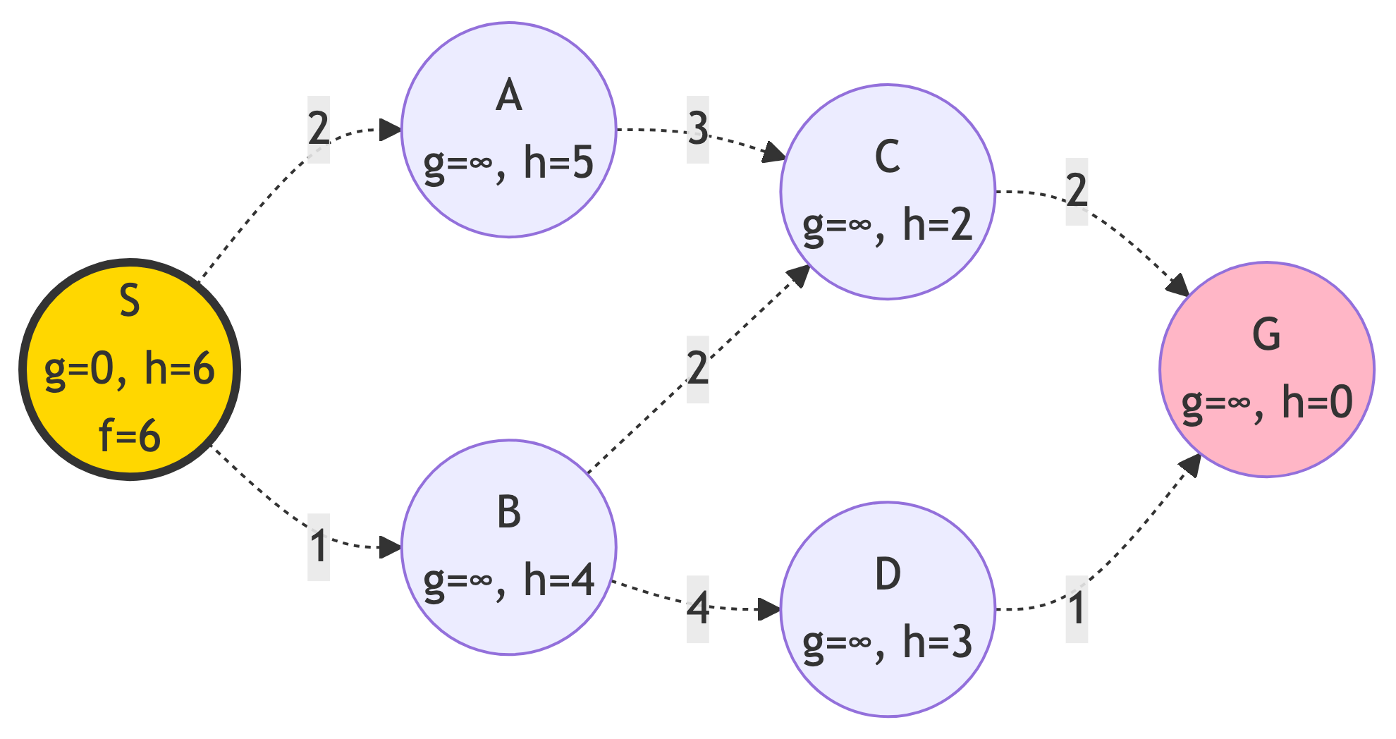
Step 0: Initialize

Starting State:

Frontier: {S (f=0+6=6)}
g-scores: {S: 0}
Explored: {}

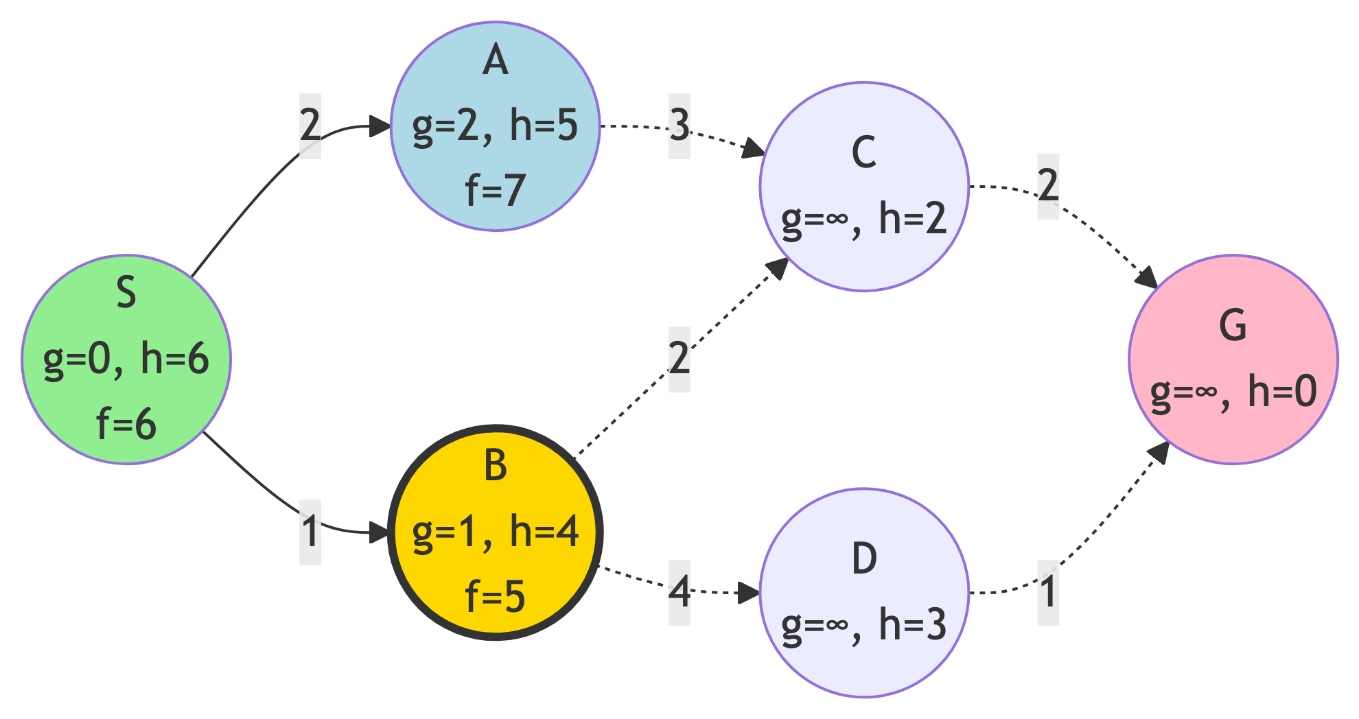
Step 1: Expand S

Action:

Calculate f-scores for neighbors

f-score Updates:

A: g=2, h=5, f=7
B: g=1, h=4, f=5

New State:

Frontier: {B (f=5), A (f=7)}
Explored: {S}

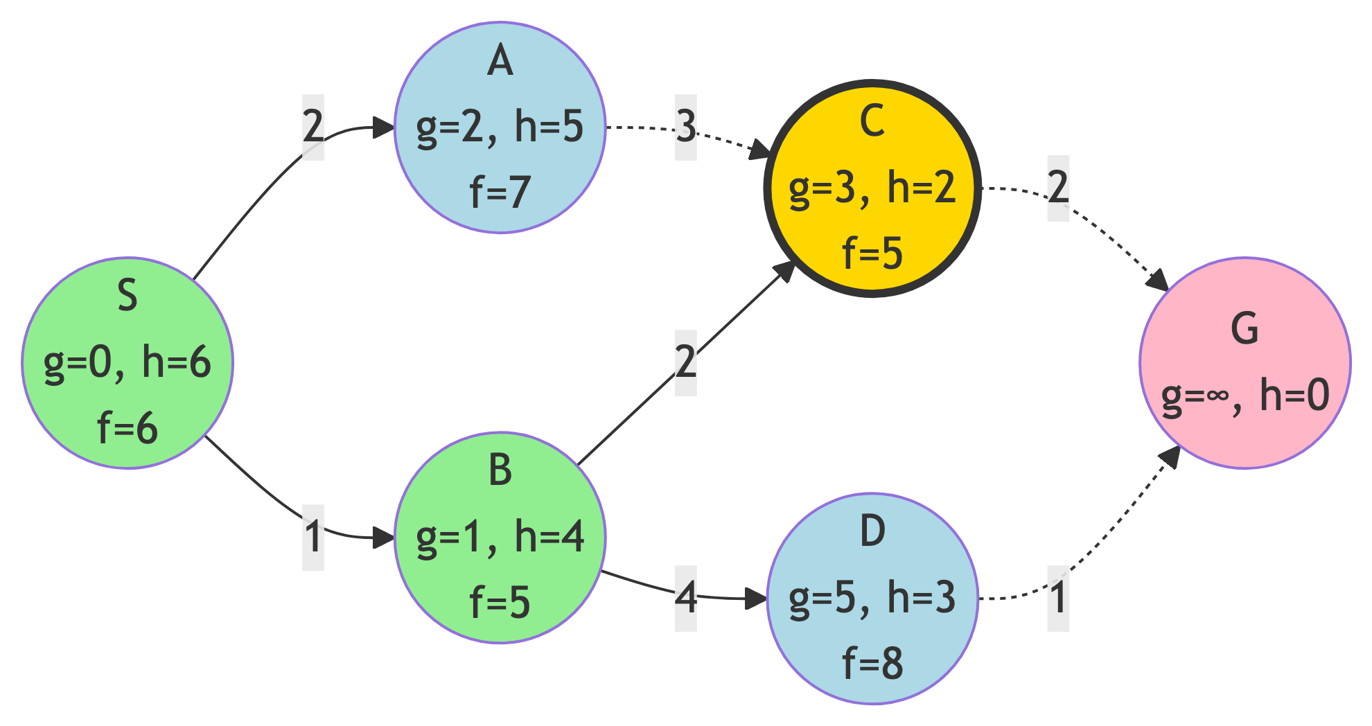
Step 2: Expand B

Action:

B has lowest f-score (f=5)

f-score Updates:

C: g=3, h=2, f=5
D: g=5, h=3, f=8

New State:

Frontier: {C (f=5), A (f=7), D (f=8)}
Explored: {S, B}

Step 3: Expand C

Action:

C has lowest f-score (f=5)

f-score Updates:

G: g=5, h=0, f=5

New State:

Frontier: {G (f=5), A (f=7), D (f=8)}
Explored: {S, B, C}

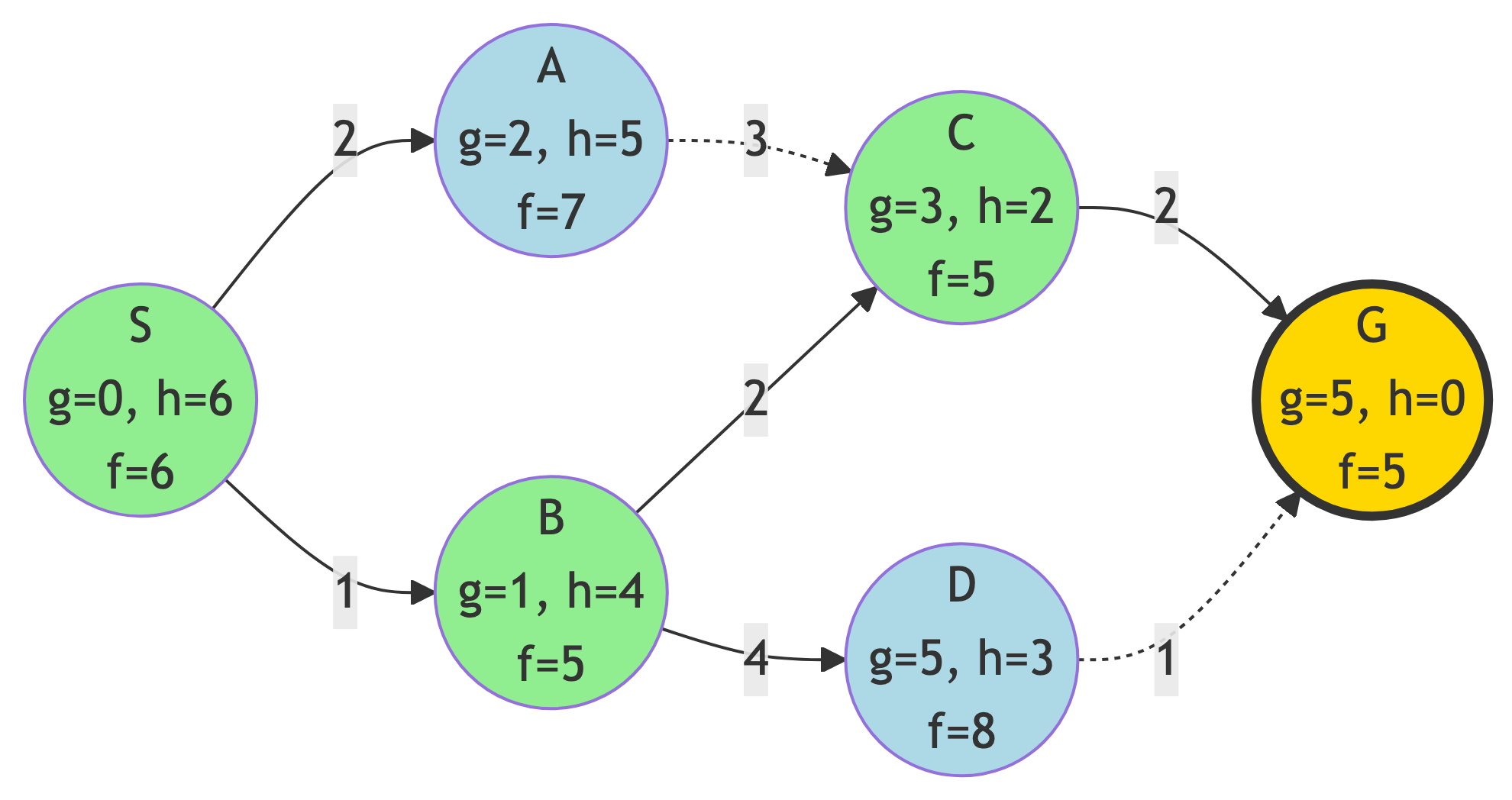
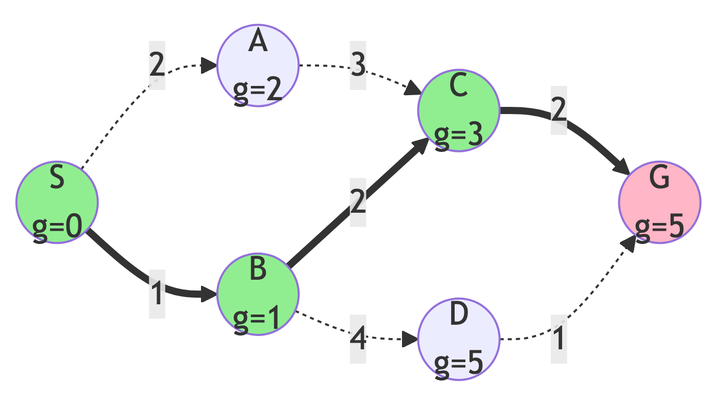
Step 4: Reach Goal

Result:

G has lowest f-score (f=5) - goal reached!

Path Found:

S → B → C → G

Path Cost:

1 + 2 + 2 = 5

A* Results

Summary:

Path: S → B → C → G
Cost: 5
Nodes Explored: 4 (S, B, C, G)
Optimal? YES (with admissible heuristic)

Observation:

A* explored the same number of nodes as Greedy BFS (4) but with the optimality guarantee of Dijkstra!

Why A* Was Efficient

The Power of f(n):

A* avoided exploring A and D because their f-scores indicated they wouldn’t lead to better solutions.

Comparison:

Node A: f=7 (higher than solution)
Node D: f=8 (higher than solution)
Solution path: all nodes had f≤5

This is why A* is often the best choice when a good heuristic is available.

Algorithm Comparison

Side-by-Side Results

Algorithm	Path	Cost	Nodes Explored	Optimal?
Greedy BFS	S→B→C→G	5	4	Yes*
Dijkstra	S→B→C→G	5	6	Yes
A*	S→B→C→G	5	4	Yes

*Greedy BFS happened to find the optimal path but doesn’t guarantee it

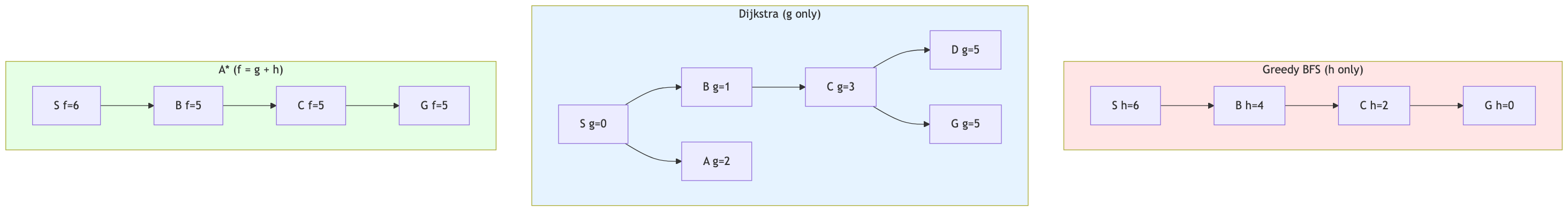
Exploration Pattern Comparison

Performance Metrics

Time Complexity:

All three: O((V + E) log V) with priority queue
In practice, efficiency varies with heuristic quality

Space Complexity:

All three: O(V) for storing nodes
A* may need more memory for f-scores

Optimality:

Greedy BFS: No guarantee
Dijkstra: Always optimal
A*: Optimal with admissible heuristic

When to Use Each Algorithm

Greedy Best-First Search:

When speed is critical and approximate solutions are acceptable
When you have a very accurate heuristic
Video games, real-time systems

Dijkstra’s Algorithm:

When optimality is required and no heuristic is available
When all edges have different costs
Network routing, GPS without traffic data

A* Search:

When optimality is required and good heuristics exist
Most pathfinding applications
GPS with traffic data, game AI, robotics

Heuristic Quality Matters

Admissible Heuristics:

Never overestimate the actual cost (h(n) ≤ actual cost)

Good Heuristics:

Lead A* to explore fewer nodes
Make A* more efficient than Dijkstra
Examples: Euclidean distance, Manhattan distance

Poor Heuristics:

If h(n) = 0 for all nodes, A* becomes Dijkstra
If h(n) overestimates, A* may not be optimal
Balance accuracy and computation time

Key Takeaways

Core Concepts

Three Different Strategies:

Greedy - Follow what looks best locally (fast, risky)
Systematic - Check everything methodically (slow, guaranteed)
Informed - Use knowledge to guide systematic search (efficient, guaranteed)

The Trade-off Triangle:

Speed ↔︎ Optimality ↔︎ Information Requirements

Practical Applications

Real-World Impact:

Google Maps uses A*-like algorithms
Video games use optimized variants for NPC pathfinding
Robots use these for navigation
Network protocols use Dijkstra variants

Choosing the Right Algorithm:

Consider your constraints and requirements before selecting an approach.