Analytic Combinatorics
CS 351: Analysis of Algorithms
Analysis of Algorithms
Charles Babbage 1840
“As soon as an Analytics Engine exists, it will necessarily guide the future course of science. Whenever any result is sought by its aid, the question will arise - By what course of calculation can these results be arrived at by the machine in the shortest time?”
Analytical Engine
Analysis of Algorithms
Ada Lovelace 1860
First computer program to calculate the Bernoulli numbers using the analytical engine.
Ada Lovelace - First Programmer

2Sum Standard Plot
# Create standard plot
fig, ax1 = plt.subplots(figsize=(10, 10))

# Standard scale plot
ax1.plot(sizes, times, 'bo-', linewidth=2, markersize=8)
ax1.set_xlabel('Input Size (N)', fontsize=12)
ax1.set_ylabel('Time (seconds)', fontsize=12)
ax1.set_title('2Sum Algorithm Performance', fontsize=14)
ax1.grid(True, alpha=0.3)

# Add annotations
for i, (x, y) in enumerate(zip(sizes, times)):
    ax1.annotate(f'({x}, {y:.2f})',
                xy=(x, y),
                xytext=(5, 5),
                textcoords='offset points',
                fontsize=9)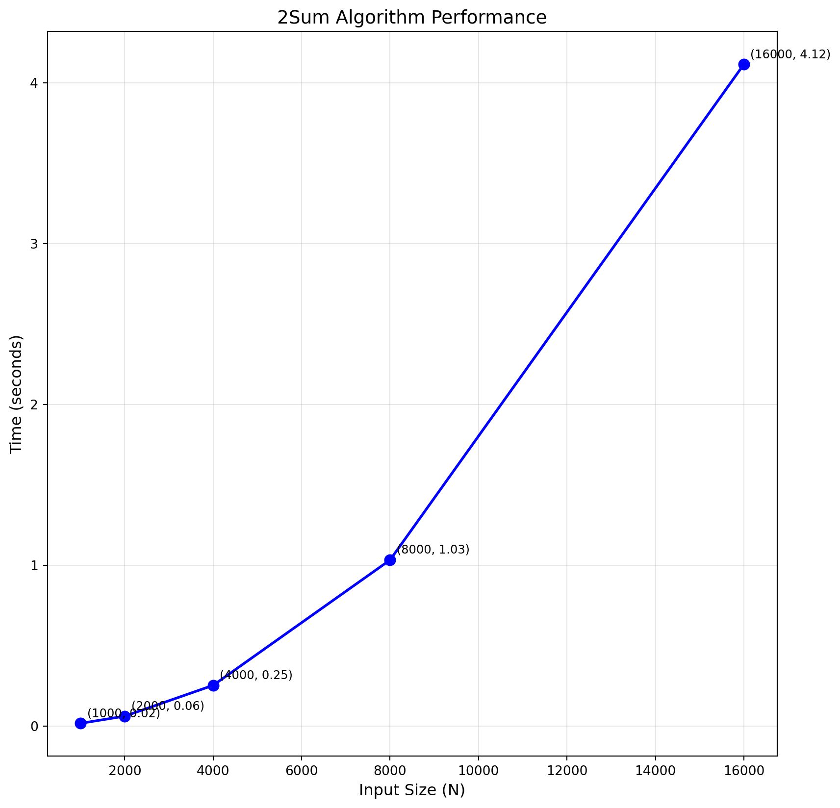
2Sum Log-Log Plot
# Log-log plot
fig, ax2 = plt.subplots(figsize=(6, 4))

ax2.loglog(sizes, times, 'ro-', linewidth=2, markersize=8, label='Empirical')
ax2.set_xlabel('Input Size (N) - log scale', fontsize=12)
ax2.set_ylabel('Time (seconds) - log scale', fontsize=12)
ax2.set_title('2Sum Log-Log Plot', fontsize=14)
ax2.grid(True, which="both", ls="-", alpha=0.2)
ax2.legend()

plt.tight_layout()
plt.show()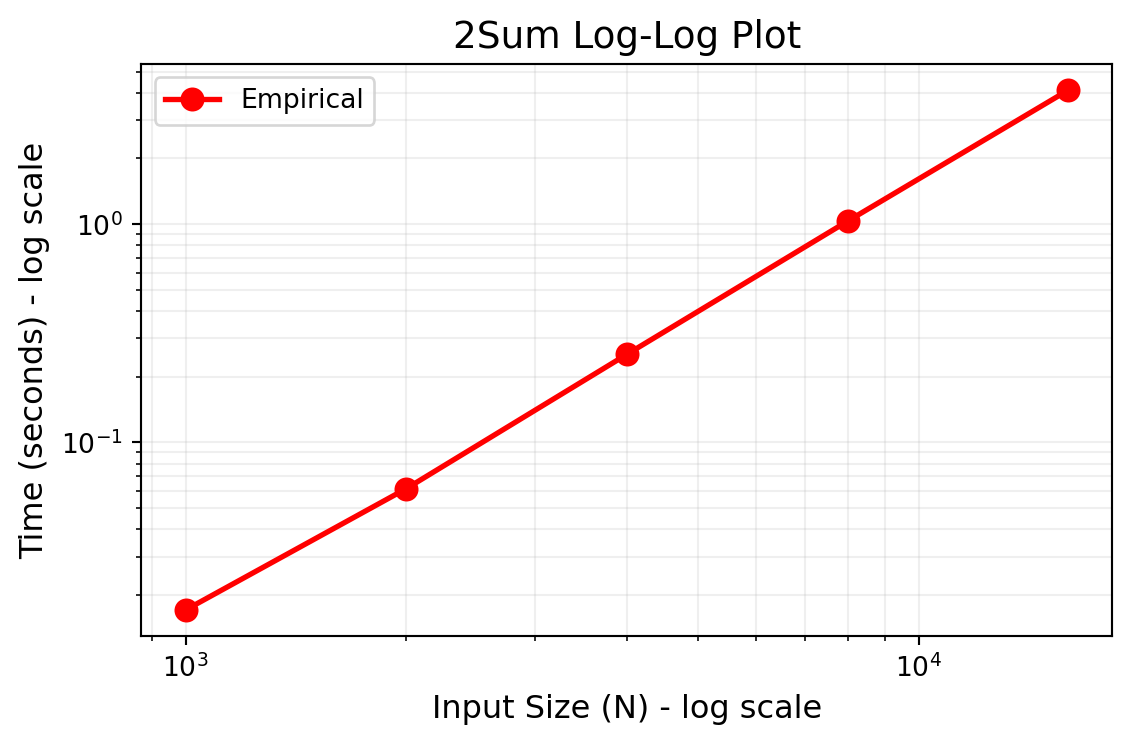
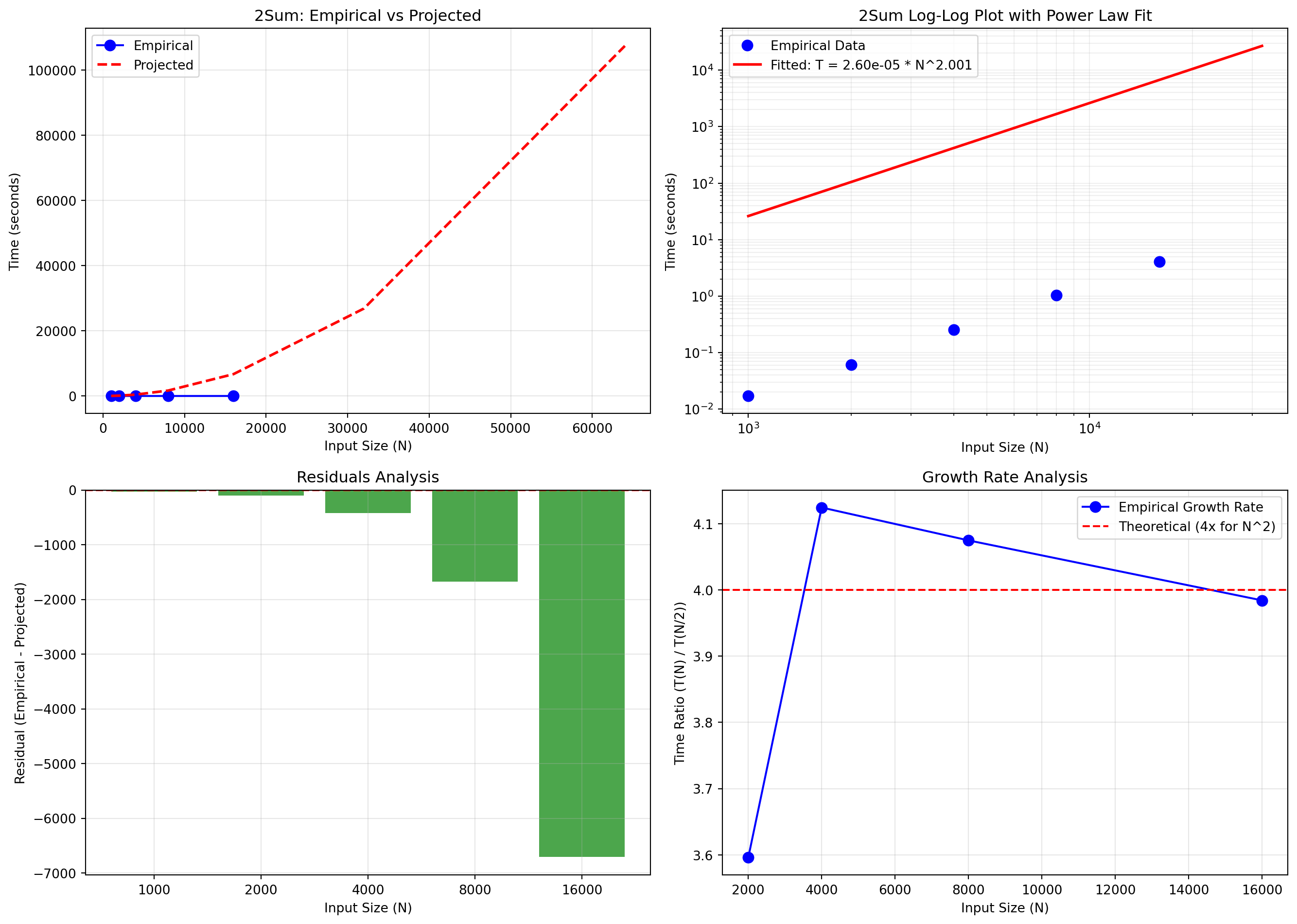
Visualize Empirical vs Projected
# Create comprehensive visualization
fig, axes = plt.subplots(2, 2, figsize=(14, 10))

# Plot 1: Standard scale with projections
ax = axes[0, 0]
ax.plot(sizes, times, 'bo-', label='Empirical', markersize=8)
extended_sizes = sizes + [32000, 64000]
extended_projected = [project_time(n, a, b) for n in extended_sizes]
ax.plot(extended_sizes, extended_projected, 'r--', label='Projected', linewidth=2)
ax.set_xlabel('Input Size (N)')
ax.set_ylabel('Time (seconds)')
ax.set_title('2Sum: Empirical vs Projected')
ax.legend()
ax.grid(True, alpha=0.3)

# Plot 2: Log-log with regression line
ax = axes[0, 1]
ax.loglog(sizes, times, 'bo', label='Empirical Data', markersize=8)
# Add regression line
N_range = np.logspace(np.log10(min(sizes)), np.log10(max(sizes)*2), 100)
T_fitted = a * N_range**b
ax.loglog(N_range, T_fitted, 'r-', label=f'Fitted: T = {a:.2e} * N^{b:.3f}', linewidth=2)
ax.set_xlabel('Input Size (N)')
ax.set_ylabel('Time (seconds)')
ax.set_title('2Sum Log-Log Plot with Power Law Fit')
ax.legend()
ax.grid(True, which="both", ls="-", alpha=0.2)

# Plot 3: Residuals
ax = axes[1, 0]
residuals = [times[i] - project_time(n, a, b) for i, n in enumerate(sizes)]
ax.bar(range(len(sizes)), residuals, color='g', alpha=0.7)
ax.set_xticks(range(len(sizes)))
ax.set_xticklabels(sizes)
ax.set_xlabel('Input Size (N)')
ax.set_ylabel('Residual (Empirical - Projected)')
ax.set_title('Residuals Analysis')
ax.axhline(y=0, color='r', linestyle='--')
ax.grid(True, alpha=0.3)

# Plot 4: Growth rate comparison
ax = axes[1, 1]
growth_rates = [times[i]/times[i-1] if i > 0 else 0 for i in range(len(times))]
theoretical_growth = [4.0] * len(sizes)  # N^2 growth means 4x when doubling
ax.plot(sizes[1:], growth_rates[1:], 'bo-', label='Empirical Growth Rate', markersize=8)
ax.axhline(y=4.0, color='r', linestyle='--', label='Theoretical (4x for N^2)')
ax.set_xlabel('Input Size (N)')
ax.set_ylabel('Time Ratio (T(N) / T(N/2))')
ax.set_title('Growth Rate Analysis')
ax.legend()
ax.grid(True, alpha=0.3)

plt.tight_layout()
plt.show()